The Christian Rationalist

I am a big fan of Google spreadsheets, and I’ve used them for a wide variety of responsibilities over the last decade or so. They’re quick, intuitive, and most importantly, easily shareable. But it’s taken me years to discover some of their most valuable features, features that have quickly become second nature for me.

Chances are, you’ve probably created a spreadsheet or two before, perhaps to manage signups for a potluck or rides to a retreat. With experience and knowledge of a few hacks, you can do so much more with them. Recently, I turned to a Google spreadsheet to display and update the schedule and standings for the church softball league I’ve been a part of, which might be able to save hundreds of dollars that we would have spent on equivalent software. Whatever your use case, there is likely something you can take away from the hacks I have to share.

1) Conditional Formatting

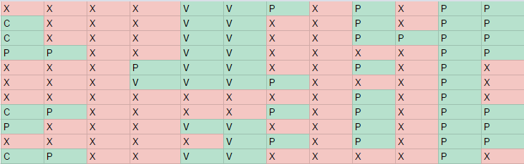
I frequently use formatting to color cells of interest to me in a spreadsheet. Coloring the background of cells gives people the general gist much more easily, and it can help to establish patterns. For instance, it’s much easier to see in this attendance chart who has been coming more or less frequently:

We were ordering pizza, so the different letters stood for what kind of pizza, if any, they wanted.

You can pick up on some attendance patterns from the first image, but they’re much clearer in color.

Rather than color each individual cell as it is filled in, though, conditional formatting allows me to color all of them in one broad stroke, taking less than a minute for the whole sheet. I simply specify the rules I want on the conditional formatting panel (accessible under Formatting, of course):

Those rules can be simple text rules like “contains ‘yes’”, or numerical rules like “is negative”. In most of the latter cases, though, I prefer to use the “color scale” option, which lets me specify a three-point scale and which automatically assigns a blend of the colors specified depending on where on that scale each value lies. For instance, in a Google spreadsheet of relevant papers in a recent literature search I did, I applied color scales to columns for the number of citations (green = 90th percentile, red = 10th percentile) and number of pages (the opposite), as well as a text-based column describing their relevance. This helped my collaborators easily see which papers were both important and easily read in the literature.

If it isn’t clear, I’ve copied part of columns F, G, and H, and shown the color scales I’ve applied to columns G and H (the color rules for column F are simple enough that you could figure them out). And no, I don’t have 1000 references; that’s just the default size of the spreadsheet.

For a while, conditional formatting was always limited to the cell you were formatting. You could format dates based on whether they were before or after today, but you couldn’t reference other cells. Then, in late 2013, Google added the “Custom formula” option to conditional formatting, which lets you do exactly that, or even write more complicated functions like coloring based on whether the cell is odd or even. The format takes some getting used to, but the key is to write the rule you want from the perspective of the first (upper leftmost) cell specified in the range. So if you want to highlight numbers that are smaller than the cell below them for the range F3:F22, you write “=F3<F4”.

My two-week projections for YouTube view counts in places 16-23 overall on May 28, 2017. If the video directly below one is going to pass it, then I shade it red, and if it’s going to pass the one above it, I shade it green, using custom formulas. There’s only one problem with this: When videos jump more than one place in two week periods, I don’t account for that. For instance, Despacito (#26 as of my predictions on May 14th) was projected to pass all of these videos into 19th place overall by May 28.

2) Using $ in formulas to freeze references to columns or rows

To save time, it’s often best to copy-paste formulas from one cell to another. However, by default, any cell references are relative: If formulas in G11 references cell A2, when copy-pasted, this simply becomes “the cell six columns to the left and nine rows up from where I am now”.

Many times, this is what you want: If you’re computing a bunch of column sums, you don’t want them all to reference the same column. But maybe there’s a special cell that enters the calculation that you don’t want to have to make a bunch of copies for just for your calculation. For instance, a component of my YouTube video projections was the date, which I always kept in the same row at the top. To always reference that date cell even if the formula is moved elsewhere, just insert a dollar sign before the column letter and/or row number. For instance, my formula for Counting Stars’ projected view count was “=M18+(P$1-L$1)*O18”. As I copy-paste that formula to other rows / videos, the references to row 18 (view count and current rate for each video) change, but the references to row 1 (the date) stay the same.

Of course, you can also put dollar signs before the letter to freeze the column being referenced. You can do both as well; this is especially useful when you’re making a table of formulas, and you want each one to reference the top cell in its column and leftmost cell in its row. You can even use $ to change the size of a range you want to reference. For instance, if you have a column of numbers in A1:A10 and you want their partial sums in the next column, you can write in B1 “=SUM(A$1:A1)” and then fill this down through B10. The top of the range will stay the same, but the end of the range will expand.

3) Linking Google Forms

Google Forms already provide a decent amount of information about the responses you’ve gotten. Without linking a Google spreadsheet, you can easily glance at the aggregate, including useful pie charts for radio (multiple choice) options and bar charts for checkboxes.

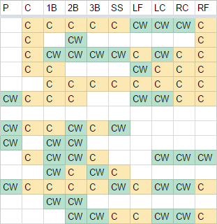
But sometimes, you want to do something more complicated with those responses, like weight them in a certain fashion or put the responses to one or two questions into an easy grid. Perhaps you want to see at a glance who wants to play each position on the softball team.

C = Can play, CW = Can and want to play. Don’t worry — this is only about half of our team.

This isn’t always as easy as it sounds, though. Suppose you want to reference the table of responses but it hasn’t been filled in yet. You might notice that when new responses come in, they don’t just fill in the rows of the new spreadsheet, but add new rows to a block above the initially empty rows. This makes them difficult to directly reference, since the rows don’t exist yet!

For formulas (like sums) referencing a range, there are a couple options: First, you could create references to a range that includes at least one more row than the block, so that the span expands as the responses are added in the middle. The other, simpler option is to delete the extra rows and use this format to reference a column all the way to the end of the spreadsheet: D$2:D. As new rows are filled in, this reference will expand to fit all of the rows.

Creating a table like the one above presents another difficulty. By default, Google Forms stores responses to checkbox questions (like “Which positions do you want to play?”) as a comma-separated list. I’ve found the easiest hack to turn this into a table is to use the REGEXMATCH function to find whether each possible answer appears in the list. You have to make sure to concatenate with “.*” (representing any character string) on either end of the REGEX so it picks up the expression wherever it occurs in the list. Here’s what one component of that formula looks like in the softball spreadsheet above:

IF(REGEXMATCH($E3,CONCATENATE(“.*”,H$1,“.*”)),“W”,“”)

4) Filter Views

Suppose you want to sort a spreadsheet without moving everything around for everyone. You could sort it and then click ‘Undo’, but then you can’t change anything, among other problems. Instead, I’d suggest using a Filter view.

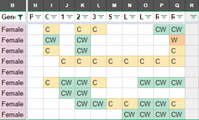
You can find Filter Views as basically their own menu under the “Data” tab — this is a bit clunky, to be honest. The first thing to do after starting a new Filter View is to make sure the range is correct: If your cursor is on a random cell, it might not grab the right range to filter on. Then you’ll notice that the top row of the range is always taken to be a header row, and you can choose whether to sort or filter according to each column. For instance, I can look at just the male or female players in the same softball spreadsheet.

Here I’ve filtered on the gender column to just pick up the female players. You’ll notice some overlaps between this table and the previous one, of course.

In additional to filtering, you can also sort according to any of those columns, in increasing or decreasing order, alphabetically or numerically. If you want to sort by multiple columns (i.e. break ties using specific columns), you actually need to go in reverse order: If you want to sort by column A, then B, then C, first sort by C, then B, then A. The latest sort always gets priority.

5) Publishing Specific Tabs

There are times when you want to release certain information to a bunch of people but keep your calculations hidden. For instance, when Grace and I were planning our wedding, we wanted people to know who else was coming so they could coordinate meeting up with each other, or decide to come if they were on the fence but saw their friends coming. We could have updated a list manually, but we didn’t want to accidentally miss anyone.

At the same time, we also didn’t want to publish all of the information guests had provided us in their RSVP. Our guests didn’t particularly need to know about each others’ dietary restrictions, for instance. Fortunately, when you publish a Google document to the web (under the File menu), you can which tabs you want to publish, and only those will be visible.

Each of those tabs were sorted by our different friend groups so they could easily find each other.

The functions SORT and FILTER are especially useful here. You can use them to copy entire ranges over, with certain columns redacted and sorted according to others. FILTER, in particular, lets you filter by rows and columns in two different ways: It filters rows by specifying some condition and which column it applies to and by columns using a simple True-False vector. (By the way, if you want to filter the opposite way, I find it easiest to use the TRANSPOSE function to flip columns and rows, apply the filter, and then apply TRANSPOSE to put it back in the original form. This is definitely a bit of a hack, but actually doesn’t make the formula that long.)

The best part of these five Google Spreadsheet hacks is that they build on each other. For my most recent softball season planning, I actually used four out of five of them: Conditional formatting to help us catch mistakes as we were laying things out, writing $’s all over the place in various formulas, linking a Google form to allow people to report scores, and publishing the final results without all of our double checks and shorthand.

With some experience and these tools, you too can create magical Google spreadsheets.